41 add or remove data labels in a chart

Add data labels, notes, or error bars to a chart - Google You can add data labels to a bar, column, scatter, area, line, waterfall, histograms, or pie chart. Learn more about chart types. On your computer, open a spreadsheet in Google Sheets. Double-click the chart you want to change. At the right, click Customize Series. Check the box next to "Data labels.". Tip: Under "Position," you can choose ... How to Customize Your Excel Pivot Chart Data Labels - dummies The Data Labels command on the Design tab's Add Chart Element menu in Excel allows you to label data markers with values from your pivot table. When you click the command button, Excel displays a menu with commands corresponding to locations for the data labels: None, Center, Left, Right, Above, and Below. None signifies that no data labels ...

How to Add Data Labels to an Excel 2010 Chart - dummies Select Number in the left pane, and then choose a number style for the data labels. Customize any additional options and then click Close. You can easily remove the data labels by clicking the Data Labels button in the Labels group on the Chart Tools Layout tab and selecting None from the drop-down menu. About This Article

Add or remove data labels in a chart

How to add data labels from different column in an Excel chart? This method will introduce a solution to add all data labels from a different column in an Excel chart at the same time. Please do as follows: 1. Right click the data series in the chart, and select Add Data Labels > Add Data Labels from the context menu to add data labels. 2. Add a DATA LABEL to ONE POINT on a chart in Excel All the data points will be highlighted. Click again on the single point that you want to add a data label to. Right-click and select ' Add data label '. This is the key step! Right-click again on the data point itself (not the label) and select ' Format data label '. You can now configure the label as required — select the content of ... Enable or Disable Excel Data Labels at the click of a button - How To Select and to go Insert tab > Charts group > Click column charts button > click 2D column chart. This will insert a new chart in the worksheet. Step 2: Having chart selected go to design tab > click add chart element button > hover over data labels > click outside end or whatever you feel fit. This will enable the data labels for the chart.

Add or remove data labels in a chart. Waterfall Charts in Excel - A Beginner's Guide | GoSkills Uncheck the Data Labels checkbox. Or Click any of the data labels. They will all be selected. Press the Delete button on your keyboard. Your chart should now look like this: How to add subtotal or total columns You'll notice that the final data point (30-Sep) is formatted and color-coded as an increase which is, of course, incorrect. Adding Data Labels to a Chart (Microsoft Word) - Tips.Net You can also use series labels as your data labels. You can add data labels to your chart by following these steps: Select Chart Options from the Chart menu. Microsoft Graph displays the Chart Options dialog box. Make sure the Data Labels tab is selected. (See Figure 1.) Figure 1. The Data Labels tab of the Chart Options dialog box How to Change Excel Chart Data Labels to Custom Values? First add data labels to the chart (Layout Ribbon > Data Labels) Define the new data label values in a bunch of cells, like this: Now, click on any data label. This will select "all" data labels. Now click once again. At this point excel will select only one data label. Go to Formula bar, press = and point to the cell where the data label ... How To Add and Remove Legends In Excel Chart? - EDUCBA The data in a chart is organized with a combination of Series and Categories. Select the chart and choose filter then you will see the categories and series. Each legend key will represent a different color to differentiate from the other legend keys. Different Actions on Legends. Now we will create a small chart and perform different actions ...

Add & edit a chart or graph - Computer - Google Docs Editors Help Double-click the chart you want to change. At the right, click Customize. Click Gridlines. Optional: If your chart has horizontal and vertical gridlines, next to "Apply to," choose the gridlines you want to change. Make changes to the gridlines. Tips: To hide gridlines but keep axis labels, use the same color for the gridlines and chart background. Change axis labels in a chart in Office - support.microsoft.com The chart uses text from your source data for axis labels. To change the label, you can change the text in the source data. If you don't want to change the text of the source data, you can create label text just for the chart you're working on. In addition to changing the text of labels, you can also change their appearance by adjusting formats. How to add or remove data labels with a click - Goodly Step 2) Place the dummy on the secondary axis Select the 2 data series (one by one) and use CTRL + 1 to open format data series box Then switch them to the secondary axis Note the secondary axis appears (we will hide that later) Step 3) Add data labels and fill the dummy with "no fill" Right click on the bar (dummy calculation) and add data labels Adding rich data labels to charts in Excel 2013 - Microsoft 365 Blog To add a data label in a shape, select the data point of interest, then right-click it to pull up the context menu. Click Add Data Label, then click Add Data Callout . The result is that your data label will appear in a graphical callout. In this case, the category Thr for the particular data label is automatically added to the callout too.

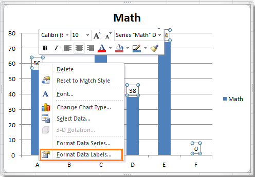
How to Add Total Data Labels to the Excel Stacked Bar Chart Apr 03, 2013 · Step 4: Right click your new line chart and select “Add Data Labels” Step 5: Right click your new data labels and format them so that their label position is “Above”; also make the labels bold and increase the font size. Step 6: Right click the line, select “Format Data Series”; in the Line Color menu, select “No line” How to add data labels to Column chart? - Stack Overflow 3 Answers. Right click on any of the bars showing on the chart that you are interested in - click 'show data labels' (Second from bottom) In the series properties, set "show data labels" to true. Point your cursor exactly to the chart (bars/column), then right click. you will see the "Show Data Labels" option. How to hide zero data labels in chart in Excel? - ExtendOffice In the Format Data Labelsdialog, Click Numberin left pane, then selectCustom from the Categorylist box, and type #""into the Format Codetext box, and click Addbutton to add it to Typelist box. See screenshot: 3. Click Closebutton to close the dialog. Then you can see all zero data labels are hidden. Add or remove data labels in a chart - support.microsoft.com Depending on what you want to highlight on a chart, you can add labels to one series, all the series (the whole chart), or one data point. Add data labels. You can add data labels to show the data point values from the Excel sheet in the chart. This step applies to Word for Mac only: On the View menu, click Print Layout.

Add data labels to a chart - Office Support

Data labels - Minitab You can add data labels to existing graphs. Double-click the graph. Right-click the graph and choose Add > Data Labels. For pie charts, choose Add > Slice Labels. Choose the label options specific to the graph and click OK. Data label options for most graphs Label the data display with y-values, row numbers, or values from a column.

How to Use Data Labels from a Range in an Excel Chart - YouTube

how to add data labels into Excel graphs - storytelling with data Right-click on a point and choose Add Data Label. You can choose any point to add a label—I'm strategically choosing the endpoint because that's where a label would best align with my design. Excel defaults to labeling the numeric value, as shown below. Now let's adjust the formatting.

Add or remove data labels in a chart - Office Support

How to Add and Remove Chart Elements in Excel Select the data, go to insert menu --> Charts --> Line Chart. 1: Add Data Label Element to The Chart To add the data labels to the chart, click on the plus sign and click on the data labels. This will ad the data labels on the top of each point. If you want to show data labels on the left, right, center, below, etc. click on the arrow sign.

Showing and Formatting Data Text Labels for All Series

Add data labels and callouts to charts in Excel 365 | EasyTweaks.com The steps that I will share in this guide apply to Excel 2021 / 2019 / 2016. Step #1: After generating the chart in Excel, right-click anywhere within the chart and select Add labels . Note that you can also select the very handy option of Adding data Callouts.

How to add or remove legends, titles or data labels in MS Excel - YouTube

Adding Data Labels to a Chart Using VBA Loops - Wise Owl To do this, add the following line to your code: 'make sure data labels are turned on. FilmDataSeries.HasDataLabels = True. This simple bit of code uses the variable we set earlier to turn on the data labels for the chart. Without this line, when we try to set the text of the first data label our code would fall over.

Add or remove data labels in a chart - Office Support

Excel tutorial: How to add and remove chart elements Chart elements can also be removed by simply selecting and deleting. Here I can click to select the data labels, and then delete. Then I can use the chart elements menu to enable the vertical axis again. It's also important to know that you can freely move many chart elements freely. Just click once to select, then over until you see the 4 ...

7 Steps to make a professional looking column graph in Excel or PowerPoint | Think Outside The Slide

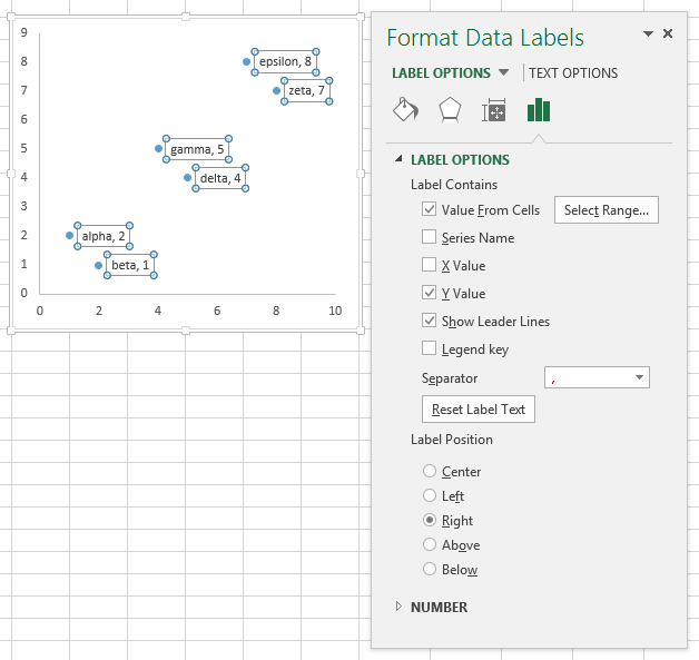
Edit titles or data labels in a chart - support.microsoft.com Right-click the data label, and then click Format Data Label or Format Data Labels. Click Label Options if it's not selected, and then select the Reset Label Text check box. Top of Page Reestablish a link to data on the worksheet On a chart, click the label that you want to link to a corresponding worksheet cell.

Surface Chart in Excel

How to use data labels in a chart - YouTube Excel charts have a flexible system to display values called "data labels". Data labels are a classic example a "simple" Excel feature with a huge range of o...

How to remove data labels from a chart in a document - YouTube

How to add or remove legends, titles or data labels in MS Excel Microsoft Excel 2007Add a chart title. Add axis titles. Link a title to a worksheet cell Add data labels. Remove titles or data labels from a chart. Show or ...

Custom data labels in a chart

Change the format of data labels in a chart To get there, after adding your data labels, select the data label to format, and then click Chart Elements > Data Labels > More Options. To go to the appropriate area, click one of the four icons ( Fill & Line, Effects, Size & Properties ( Layout & Properties in Outlook or Word), or Label Options) shown here.

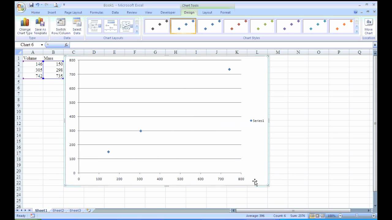
X-Y scatter plot in Excel 2007 - YouTube

How to add or move data labels in Excel chart? - ExtendOffice 1. Click the chart to show the Chart Elements button . 2. Then click the Chart Elements, and check Data Labels, then you can click the arrow to choose an option about the data labels in the sub menu. See screenshot: In Excel 2010 or 2007. 1. click on the chart to show the Layout tab in the Chart Tools group. See screenshot: 2.

Apply Custom Data Labels to Charted Points - Peltier Tech Blog

Add / Move Data Labels in Charts - Excel & Google Sheets Add and Move Data Labels in Google Sheets Double Click Chart Select Customize under Chart Editor Select Series 4. Check Data Labels 5. Select which Position to move the data labels in comparison to the bars. Final Graph with Google Sheets After moving the dataset to the center, you can see the final graph has the data labels where we want.

Resize the Plot Area in Excel Chart - Titles and Labels Overlap - YouTube

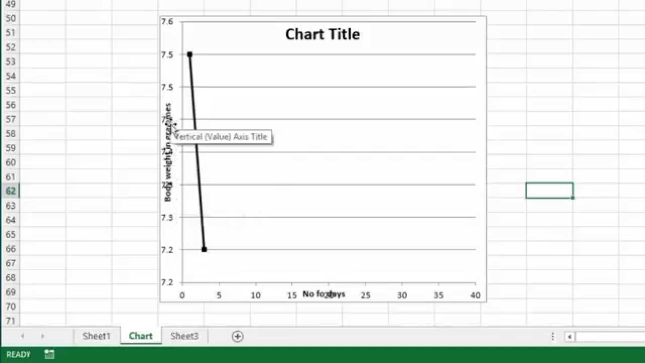
Add or remove titles in a chart - support.microsoft.com To remove a chart title, on the Layout tab, in the Labels group, click Chart Title, and then click None. To remove an axis title, on the Layout tab, in the Labels group, click Axis Title , click the type of axis title that you want to remove, and then click None .

How to hide zero data labels in chart in Excel?

Enable or Disable Excel Data Labels at the click of a button - How To Select and to go Insert tab > Charts group > Click column charts button > click 2D column chart. This will insert a new chart in the worksheet. Step 2: Having chart selected go to design tab > click add chart element button > hover over data labels > click outside end or whatever you feel fit. This will enable the data labels for the chart.

Nabu Press Lehrbuch der politischen Oekonomie, F?nfter Band (German Edition) | massgenie.com

Add a DATA LABEL to ONE POINT on a chart in Excel All the data points will be highlighted. Click again on the single point that you want to add a data label to. Right-click and select ' Add data label '. This is the key step! Right-click again on the data point itself (not the label) and select ' Format data label '. You can now configure the label as required — select the content of ...